F-IF Logistic Growth Model, Abstract Version
An important example of a model often used in biology or ecology to model population growth is called the logistic growth model. The general form of the logistic equation is $$ P(t) = \frac{KP_0e^{rt}}{K+P_0(e^{rt}-1)}. $$ In this equation \(t\) represents time, with \(t = 0\) corresponding to when the population in question is first measured; \(K,P_0\) and \(r\) are all real numbers with \(K\) being called the ``carrying capacity'' while \(r\) is a growth rate and is normally a positive number.
- Explain why the value \(P_0\) represents the population when it is first measured.
- Explain why, as time elapses, the population stabilizes, approaching the value \(K\).
- Explain how the behavior of \(P\) changes if the growth rate \(r\) is increased or decreased.
- Below is the graph of a particular logistic function \(P\), showing the growth of a bacteria population. Using the graph, identify \(P_0\) and \(K\).
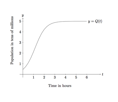
- Using the values of \(P_0\) and \(K\) from the previous part, sketch the graph of the logistic function \(Q\) given by $$ Q(t) = \frac{KP_0e^{2rt}}{K+P_0(e^{2rt}-1)}. $$ Note that \(Q\) is the same as \(P\) except that the growth rate \(r\) has been doubled.

Solutions
- The population is first measured when \(t = 0\). Plugging \(t = 0\) into the expression for \(P\) gives \begin{align} P(0) &= \frac{KP_0e^{r \cdot 0}}{K + P_0(e^{r \cdot 0} - 1)} \\ &= \frac{KP_0e^0}{K + P_0(e^0 - 1)} \\ &= \frac{KP_0}{K} \\ &= P_0. \end{align}
- As the name suggests, the ``carrying capacity'' is the maximum population that the environment can sustain so it is, in this case, the value that the population approaches as \(t\) grows. Expanding the expression for the denominator of \(P\), \(K - P_0e^{rt} - P_0\), the exponential term \(P_0e^{rt}\), grows rapidly as \(t\) grows. The rest of the denominator, \(K - P_0\), does not depend on \(t\). So as \(t\) grows, the denominator is better and better approximated by \(P_0e^{rt}\). The numerator is \(KP_0e^{rt}\). Taking the quotient of \(KP_0e^{rt}\) by \(P_0e^{rt}\) gives \(K\), the carrying capacity. So as \(t\) grows, the values of \(P\) become closer and closer to \(K\).
- The rate \(r\) determines how quickly the exponential function \(e^{rt}\) grows. Increasing \(r\) will increase the rate of growth of \(e^{rt}\). This means that the values of \(P\) will approach the carrying capacity \(K\) more rapidly since, as seen in part (b), it is the growth of the \(e^{rt}\) term that make the population approach \(K\). If \(r\) is decreased, then \(e^{rt}\) grows more slowly and the values of \(P\) approach \(K\) more slowly.
-
The value \(P(0)\) is the \(y\)-intercept of the graph of \(P\). This value is about half way between \(0\) and \(1\) and since the units in population for the graph are \(10\) million this means that there are about \(5\) million bacteria at the beginning of the experiment. The carrying capacity \(K\) appears to be close to \(5\) which represents \(50\) million bacteria.
If the actual formula for the function is given, then the \(y\)-intercept can be calculated exactly $$ P(0) = \frac{5 e^{0}}{1 + 10e^{0}} = \frac{5}{11}. $$ Since one unit on the graph represents \(10,000,000\) bacteria, there are a little under \(5\) million bacteria when the population is first measured. The carrying capacity is \(50,000,000\) as estimated above: since the \(e^{-t}\) term, in the population formula, becomes less and less significant as \(t\) grows the population approaches \(\frac{5}{1}\) units or \(50,000,000\).
-
When the value \(r\) is doubled, looking at part (b), what this means is that the exponential term \(P_0e^{2 rt}\) in the denominator becomes the dominant term more quickly, twice as quickly in fact. So we expect the population to grow more rapidly at the beginning before approaching the carrying capacity. This is shown in the graph below. Note that this graph is precise because the precise values of \(K, P_0,\) and \(r\) were used: not knowing this information the best one can do is draw a curve with the same initial population, the same carrying capacity, and which grows more rapidly initially.
Commentary
This task is for instructional purposes only and students should already be familiar with some specific examples of logistic growth functions such as that given in ``Logistic growth model, concrete case.'' This is an important example of a function with many constants: \(P_0\) the initial population, \(K\) the carrying capacity, and \(r\) the growth rate. Each of these has a specific meaning which determines the shape of the graph and, in case of \(P_0\) and \(K\), can be readily estimated using the graph.
The goal of this task is to have students appreciate how the different constants (\(P_0\), \(K\), and \(r\)) influence the shape of the graph. Only \(r\) has been changed here, in part (e), because it is the most abstract of these numbers. If the instructor wishes to change the other numbers, the function used to generate this particular graph is $$ P(t) = \frac{5}{1 + 10e^{-t}}. $$ Note that this is not given in the form of the logistic equation given above with \(K,P_0,\) and \(r\). It corresponds, after algebraic manipulation, to the case where \(r = 1\), \(K = 5\), \(P_0 = \frac{5}{11}\). Showing this identity is a worthwhile algebraic exercise which requires careful manipulation of fractions and exponential functions.