Acceleration and Free Fall
Article objectives
The motion of falling objects
The motion of falling objects is the simplest and most common example of motion with changing velocity. The early pioneers of physics had a correct intuition that the way things drop was a message directly from Nature herself about how the universe worked. Other examples seem less likely to have deep significance. A walking person who speeds up is making a conscious choice. If one stretch of a river flows more rapidly than another, it may be only because the channel is narrower there, which is just an accident of the local geography. But there is something impressively consistent, universal, and inexorable about the way things fall.
Stand up now and simultaneously drop a coin and a bit of paper side by side. The paper takes much longer to hit the ground. That's why Aristotle wrote that heavy objects fell more rapidly. Europeans believed him for two thousand years.
Now repeat the experiment, but make it into a race between the coin and your shoe. It looks like they hit the ground at exactly the same moment. Galileo, who had a flair for the theatrical, did the experiment by dropping a bullet and a heavy cannonball from a tall tower. Aristotle's observations had been incomplete, his interpretation a vast oversimplification.
It is inconceivable that Galileo was the first person to observe a discrepancy with Aristotle's predictions. Galileo was the one who changed the course of history because he was able to assemble the observations into a coherent pattern, and also because he carried out systematic quantitative (numerical) measurements rather than just describing things qualitatively.
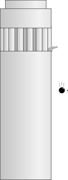
Figure a: Galileo dropped a cannonball and a musketball simultaneously from a tower, and observed that they hit the ground at nearly the same time. This contradicted Aristotle's long-accepted idea that heavier objects fell faster.
Why is it that some objects, like the coin and the shoe, have similar motion, but others, like a feather or a bit of paper, are different? Galileo speculated that in addition to the force that always pulls objects down, there was an upward force exerted by the air. Anyone can speculate, but Galileo went beyond speculation and came up with two clever experiments to probe the issue. First, he experimented with objects falling in water, which probed the same issues but made the motion slow enough that he could take time measurements with a primitive pendulum clock. With this technique, he established the following facts:
-
All heavy, streamlined objects (for example a steel rod dropped point-down) reach the bottom of the tank in about the same amount of time, only slightly longer than the time they would take to fall the same distance in air.
-
Objects that are lighter or less streamlined take a longer time to reach the bottom.
This supported his hypothesis about two contrary forces. He imagined an idealized situation in which the falling object did not have to push its way through any substance at all. Falling in air would be more like this ideal case than falling in water, but even a thin, sparse medium like air would be sufficient to cause obvious effects on feathers and other light objects that were not streamlined. Today, we have vacuum pumps that allow us to suck nearly all the air out of a chamber, and if we drop a feather and a rock side by side in a vacuum, the feather does not lag behind the rock at all.

Figure b: Velocity increases more gradually on the gentle slope, but the motion is otherwise the same as the motion of a falling object.

Figure c: The v-t graph of a falling object is a line.
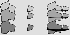 Figure d: Galileo's experiments show that all falling objects have the same motion if air resistance is negligible.
How the speed of a falling object increases with time
Galileo's second stroke of genius was to find a way to make quantitative measurements of how the speed of a falling object increased as it went along. Again it was problematic to make sufficiently accurate time measurements with primitive clocks, and again he found a tricky way to slow things down while preserving the essential physical phenomena: he let a ball roll down a slope instead of dropping it vertically. The steeper the incline, the more rapidly the ball would gain speed. Without a modern video camera, Galileo had invented a way to make a slow-motion version of falling.
Although Galileo's clocks were only good enough to do accurate experiments at the smaller angles, he was confident after making a systematic study at a variety of small angles that his basic conclusions were generally valid. Stated in modern language, what he found was that the velocity-versus-time graph was a line. In the language of algebra, we know that a line has an equation of the form y=ax+b, but our variables are v and t, so it would be v=at+b. (The constant b can be interpreted simply as the initial velocity of the object, i.e., its velocity at the time when we started our clock, which we conventionally write as v\(_{o}\).)
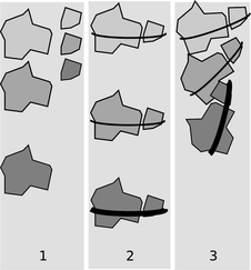
Figure e: 1. Aristotle said that heavier objects fell faster than lighter ones. 2. If two rocks are tied together, that makes an extra- heavy rock, which should fall faster. 3. But Aristotle's theory would also predict that the light rock would hold back the heavy rock, resulting in a slower fall.
A contradiction in Aristotle's reasoning
Galileo's inclined-plane experiment disproved the long-accepted claim by Aristotle that a falling object had a definite “natural falling speed” proportional to its weight. Galileo had found that the speed just kept on increasing, and weight was irrelevant as long as air friction was negligible. Not only did Galileo prove experimentally that Aristotle had been wrong, but he also pointed out a logical contradiction in Aristotle's own reasoning. Simplicio, the stupid character, mouths the accepted Aristotelian wisdom:
Simplicio: There can be no doubt but that a particular body ... has a fixed velocity which is determined by nature...
Salviati: If then we take two bodies whose natural speeds are different, it is clear that, [according to Aristotle], on uniting the two, the more rapid one will be partly held back by the slower, and the slower will be somewhat hastened by the swifter. Do you not agree with me in this opinion?
Simplicio: You are unquestionably right.
Salviati: But if this is true, and if a large stone moves with a speed of, say, eight [unspecified units] while a smaller moves with a speed of four, then when they are united, the system will move with a speed less than eight; but the two stones when tied together make a stone larger than that which before moved with a speed of eight. Hence the heavier body moves with less speed than the lighter; an effect which is contrary to your supposition. Thus you see how, from your assumption that the heavier body moves more rapidly than the lighter one, I infer that the heavier body moves more slowly.
What is gravity?
The physicist Richard Feynman liked to tell a story about how when he was a little kid, he asked his father, “Why do things fall?” As an adult, he praised his father for answering, “Nobody knows why things fall. It's a deep mystery, and the smartest people in the world don't know the basic reason for it.” Contrast that with the average person's off-the-cuff answer, “Oh, it's because of gravity.” Feynman liked his father's answer, because his father realized that simply giving a name to something didn't mean that you understood it. The radical thing about Galileo's and Newton's approach to science was that they concentrated first on describing mathematically what really did happen, rather than spending a lot of time on untestable speculation such as Aristotle's statement that “Things fall because they are trying to reach their natural place in contact with the earth.” That doesn't mean that science can never answer the “why” questions. Over the next month or two as you delve deeper into physics, you will learn that there are more fundamental reasons why all falling objects have v-t graphs with the same slope, regardless of their mass. Nevertheless, the methods of science always impose limits on how deep our explanation can go.
Definition of acceleration for linear v-t graphs

Figure f: Example 1.

Figure g: Example 2.
Galileo's experiment with dropping heavy and light objects from a tower showed that all falling objects have the same motion, and his inclined-plane experiments showed that the motion was described by v=at+v\(_{o}\). The initial velocity v\(_{o}\) depends on whether you drop the object from rest or throw it down, but even if you throw it down, you cannot change the slope, a, of the v-t graph.
Since these experiments show that all falling objects have linear v-t graphs with the same slope, the slope of such a graph is apparently an important and useful quantity. We use the word acceleration, and the symbol a, for the slope of such a graph. In symbols, a=Δ v/Δt. The acceleration can be interpreted as the amount of speed gained in every second, and it has units of velocity divided by time, i.e., “meters per second per second,” or m/s/s. Continuing to treat units as if they were algebra symbols, we simplify “m/s/s” to read m/s\(^{2}\).” Acceleration can be a useful quantity for describing other types of motion besides falling, and the word and the symbol “a” can be used in a more general context. We reserve the more specialized symbol “g” for the acceleration of falling objects, which on the surface of our planet equals 9.8 m/s\(^{2}\) . Often when doing approximate calculations or merely illustrative numerical examples it is good enough to use g=10 m/s\(^{2}\) , which is off by only 2%.
Example 1 Finding final speed, given time
◊ A despondent physics student jumps off a bridge, and falls for three seconds before hitting the water. How fast is he going when he hits the water?
◊ Approximating g as 10 m/s\(^{2}\) , he will gain 10 m/s of speed each second. After one second, his velocity is 10 m/s, after two seconds it is 20 m/s, and on impact, after falling for three seconds, he is moving at 30 m/s.
Example 2 Extracting acceleration from a graph
◊ The x-t and v-t graphs show the motion of a car starting from a stop sign. What is the car's acceleration? ◊ Acceleration is defined as the slope of the v-t graph. The graph rises by 3 m/s during a time interval of 3 s, so the acceleration is (3 m/s)/(3 s)=1 m/s\(^{2}\) .
Incorrect solution #1: The final velocity is 3 m/s, and acceleration is velocity divided by time, so the acceleration is (3 m/s)/(10 s)=0.3 m/s\(^{2}\) The solution is incorrect because you can't find the slope of a graph from one point. This person was just using the point at the right end of the v-t graph to try to find the slope of the curve.
Incorrect solution #2: Velocity is distance divided by time so v=(4.5 m)/(3 s)=1.5 m/s. Acceleration is velocity divided by time, so a=(1.5 m/s)/(3 s)=0.5 m/s\(^{2}\) . The solution is incorrect because velocity is the slope of the tangent line. In a case like this where the velocity is changing, you can't just pick two points on the x-t graph and use them to find the velocity.
Example 3 Converting g to different units
◊ What is g in units of cm/s\(^{2}\) ?
◊ The answer is going to be how many cm/s of speed a falling object gains in one second. If it gains 9.8 m/s in one second, then it gains 980 cm/s in one second, so g=980 cm/s2 . Alternatively, we can use the method of fractions that equal one:
$$9.8 m/s^2×100 cm/1 m=980 cm/s^2$$
◊ What is g in units of miles/hour\(^{2}\)?
◊
$$9.8 m/s^2×1 mile/1600 m×(3600 s/1 hour)2=7.9×10⁴ mile/hour^2$$
This large number can be interpreted as the speed, in miles per hour, that you would gain by falling for one hour. Note that we had to square the conversion factor of 3600 s/hour in order to cancel out the units of seconds squared in the denominator.
◊ What is g in units of miles/hour/s?
$$9.8 m/s^2×1 mile/1600 m×3600 s/1 hour=22 mile/hour/s$$
This is a figure that Americans will have an intuitive feel for. If your car has a forward acceleration equal to the acceleration of a falling object, then you will gain 22 miles per hour of speed every second. However, using mixed time units of hours and seconds like this is usually inconvenient for problem-solving. It would be like using units of foot-inches for area instead of ft\(^{2}\) or in\(^{2}\).
The acceleration of gravity is different in different locations. Everyone knows that gravity is weaker on the moon, but actually it is not even the same everywhere on Earth, as shown by the sampling of numerical data in the following table.
| $$\text{Location}$$ | $$\text{Latitude}$$ | $$\text{Elevation (m)}$$ | $$g (m/s^2)$$ | |
|---|---|---|---|---|
| North Pole | $$90^\circ N$$ | 0 | 9.8322 | |
| Reykjavik, Iceland | $$64^\circ N$$ | 0 | 9.8225 | |
| Guayaquil, Ecuador | $$2^\circ S$$ | 0 | 9.7806 | |
| Mt. Cotopaxi, Ecuador | $$1^\circ S$$ | 5896 | 9.7624 | |
| Mt. Everest | $$28^\circ N$$ | 8848 | 9.7643 |
The main variables that relate to the value of g on Earth are latitude and elevation. Although you have not yet learned how g would be calculated based on any deeper theory of gravity, it is not too hard to guess why g depends on elevation. Gravity is an attraction between things that have mass, and the attraction gets weaker with increasing distance. As you ascend from the seaport of Guayaquil to the nearby top of Mt. Cotopaxi, you are distancing yourself from the mass of the planet. The dependence on latitude occurs because we are measuring the acceleration of gravity relative to the earth's surface, but the earth's rotation causes the earth's surface to fall out from under you.

Figure h: This false-color map shows variations in the strength of the earth's gravity. Purple areas have the strongest gravity, yellow the weakest. The overall trend toward weaker gravity at the equator and stronger gravity at the poles has been artificially removed to allow the weaker local variations to show up. The map covers only the oceans because of the technique used to make it: satellites look for bulges and depressions in the surface of the ocean. A very slight bulge will occur over an undersea mountain, for instance, because the mountain's gravitational attraction pulls water toward it. The US government originally began collecting data like these for military use, to correct for the deviations in the paths of missiles. The data have recently been released for scientific and commercial use (e.g., searching for sites for off-shore oil wells).
Much more spectacular differences in the strength of gravity can be observed away from the Earth's surface:
\(\text{Location g (m/s\(^{2}\))}\)
asteroid Vesta (surface) 0.3
Earth’s moon (surface) 1.6
Mars (surface) 3.7
Earth (surface) 9.8
Jupiter (cloud-tops) 26
Sun (visible surface) 270
typical neutron star (surface) 1012
black hole (center) infinite according to some theories, on the order of 1052 according to others
A typical neutron star is not so different in size from a large asteroid, but is orders of magnitude more massive, so the mass of a body definitely correlates with the g it creates. On the other hand, a neutron star has about the same mass as our Sun, so why is its g billions of times greater? If you had the misfortune of being on the surface of a neutron star, you'd be within a few thousand miles of all its mass, whereas on the surface of the Sun, you'd still be millions of miles from most of its mass.
\(\text{Positive and Negative Acceleration}\)
Gravity always pulls down, but that does not mean it always speeds things up. If you throw a ball straight up, gravity will first slow it down to v=0 and then begin increasing its speed. People often get the impression that positive signs of acceleration indicated speeding up, while negative accelerations represented slowing down, i.e., deceleration. Such a definition would be inconvenient, however, because we would then have to say that the same downward tug of gravity could produce either a positive or a negative acceleration. As we will see in the following example, such a definition also would not be the same as the slope of the v-t graph.
Let's study the example of the rising and falling ball. In the example of the person falling from a bridge, positive velocity values are assumed without calling attention to it, which meant that the coordinate system is one whose x axis pointed down. In this example, where the ball is reversing direction, it is not possible to avoid negative velocities by a tricky choice of axis, so let's make the more natural choice of an axis pointing up. The ball's velocity will initially be a positive number, because it is heading up, in the same direction as the x axis, but on the way back down, it will be a negative number. As shown in the figure, the v-t graph does not do anything special at the top of the ball's flight, where v equals 0. Its slope is always negative. In the left half of the graph, there is a negative slope because the positive velocity is getting closer to zero. On the right side, the negative slope is due to a negative velocity that is getting farther from zero, so we say that the ball is speeding up, but its velocity is decreasing!

Figure i: The ball's acceleration stays the same --- on the way up, at the top, and on the way back down. It's always negative.
To summarize, what makes the most sense is to stick with the original definition of acceleration as the slope of the v-t graph, Δ v/Δ t. By this definition, it just isn't necessarily true that things speeding up have positive acceleration while things slowing down have negative acceleration. The word “deceleration” is not used much by physicists, and the word “acceleration” is used unblushingly to refer to slowing down as well as speeding up: “There was a red light, and we accelerated to a stop.”
Example 4 Numerical calculation of a negative acceleration
◊In figure i, what happens if you calculate the acceleration between \(t=1.0\) and \(1.5 \; s\)?
◊ Reading from the graph, it looks like the velocity is about -1 m/s at \(t=1.0 \; s\), and around \(-6 m/s\) at \(t=1.5 s\). The acceleration, figured between these two points, is
$$a = Δv/Δt= (-6 \frac{m}{s}) - (-1 \frac{m}{s})(1.5 \; s) - (1.0 \; s) = -10 \frac{m}{s^2}$$
Even though the ball is speeding up, it has a negative acceleration. This is because the velocity is increasing relative to the negative vertical axis, so we write the acceleration as a negative quantity.
Another way of convincing you that this way of handling the plus and minus signs makes sense is to think of a device that measures acceleration. After all, physics is supposed to use operational definitions, ones that relate to the results you get with actual measuring devices. Consider an air freshener hanging from the rear-view mirror of your car. When you speed up, the air freshener swings backward. Suppose we define this as a positive reading. When you slow down, the air freshener swings forward, so we'll call this a negative reading on our accelerometer. But what if you put the car in reverse and start speeding up backwards? Even though you're speeding up, the accelerometer responds in the same way as it did when you were going forward and slowing down. There are four possible cases:
| $$\text{Motion of car}$$ | $$\text{Accelerometer Swings}$$ | $$\text{Slope of *v-t* graph}$$ | Direction of force acting on car | |
|---|---|---|---|---|
| Forward, speeding up | Backward | + | Forward | |
| Forward, slowing down | Forward | - | Backward | |
| Backward, speeding up | Forward | - | Backward | |
| Backward, slowing down | Backward | + | Forward |
Note the consistency of the three right-hand columns --- nature is trying to tell us that this is the right system of classification, not the left-hand column.
Because the positive and negative signs of acceleration depend on the choice of a coordinate system, the acceleration of an object under the influence of gravity can be either positive or negative. Rather than having to write things like “ g=9.8 m/s\(^{2}\) or -9.8 m/s\(^{2}\) ” every time we want to discuss g's numerical value, we simply define g as the absolute value of the acceleration of objects moving under the influence of gravity. We consistently let g=9.8 m/s\(^{2}\) , but we may have either a=g or a=-g, depending on our choice of a coordinate system.
Example 5 Acceleration with a change in direction of motion
◊ A person kicks a ball, which rolls up a sloping street, comes to a halt, and rolls back down again. The ball has constant acceleration. The ball is initially moving at a velocity of 4.0 m/s, and after 10.0 s it has returned to where it started. At the end, it has sped back up to the same speed it had initially, but in the opposite direction. What was its acceleration?
◊ By giving a positive number for the initial velocity, the statement of the question implies a coordinate axis that points up the slope of the hill. The “same” speed in the opposite direction should therefore be represented by a negative number, -4.0 m/s. The acceleration is
$$a =Δv/Δt =(v_f-v_o)/10.0 s =[(-4.0 m/s)-(4.0 m/s)]/10.0s =-0.80 m/s^2$$
The acceleration was no different during the upward part of the roll than on the downward part of the roll.
Incorrect solution: Acceleration is Δ v/Δt, and at the end it's not moving any faster or slower than when it started, so Δv=0 and a=0.
The velocity does change, from a positive number to a negative number.
Here is a different example involving free fall equations.
Example 6: A beanbag undergoes free fall for 3 seconds. If we ignore air resistance and assume the beanbag does not hit anything while in free fall, find the final velocity of the beanbag in terms of the initial velocity.
Solution: Define the positive y-axis to be upward in space; therefore the negative y-axis points towards the ground. Air resistance is ignored, so \(a = g\). Since \(g\) is a constant, we consider equations where the acceleration is constant. One equation that has both of the variables we need in our final equation is
$$v_f^2 = v_0^2 + 2g(y - y_0)$$
We can substitute in \(g\) right away:
$$v_f^2 = v_0^2 + 2(9.8)(y - y_0) \Rightarrow$$ $$v_f^2 = v_0^2 - 19.6(y - y_0)$$
We have no information on the value of \(y\) or \(y_0\). This is where introducing another equation will be useful. Consider this other equation for constant acceleration in free fall:
$$y = y_0 + v_0t + \frac{1}{2}gt^2$$
Insert the values for \(g\) and \(t\):
$$y = y_0 + v_0(3) + \frac{1}{2}(-9.8)(3)^2 \Rightarrow$$ $$y = y_0 + 3v_0 - 4.9(9) \Rightarrow$$ $$y = y_0 + 3v_0 - 44.1$$
This is useful because we can subtract \(y_0\) from both sides of the equation:
$$y - y_0 = 3v_0 - 44.1$$
The right side only involves the initial velocity, meaning a smart move would be to substitute into the first equation we broke down:
$$v_f^2 = v_0^2 - 19.6(3v_0 - 44.1) \Rightarrow$$ $$v_f^2 = v_0^2 - 5.88v_0 + 864.36$$
Take the square root of both sides of the equation:
$$v_f = \pm \sqrt{v_0^2 - 5.88v_0 + 864.36}$$
However, the beanbag is falling in the negative y-direction, so the velocity must be negative. Therefore
$$v_f = -\sqrt{v_0^2 - 5.88v_0 + 864.36}$$
Varying Acceleration
So far we have only been discussing examples of motion for which the v-t graph is linear. If we wish to generalize our definition to v-t graphs that are more complex curves, the best way to proceed is similar to how we defined velocity for curved x-t graphs:
definition of acceleration The acceleration of an object at any instant is the slope of the tangent line passing through its v-versus-t graph at the relevant point.
Example 7 A skydiver

Figure j: Example 7.
◊ The graphs in figure k show the results of a fairly realistic computer simulation of the motion of a skydiver, including the effects of air friction. The x axis has been chosen pointing down, so x is increasing as she falls. Find (a) the skydiver's acceleration at t=3.0 s , and also (b) at t=7.0 s . ◊ The solution is shown in figure l. I've added tangent lines at the two points in question.
(a) To find the slope of the tangent line, pick two points on the line (not necessarily on the actual curve): (3.0 s, 28m/s) and (5.0 s,42 m/s) . The slope of the tangent line is (42 m/s-28 m/s)/(5.0 s-3.0 s)=7.0 m/s\(^{2}\) .
(b) Two points on this tangent line are (7.0 s,47 m/s) and (9.0 s,52 m/s) . The slope of the tangent line is (52 m/s-47 m/s)/(9.0 s-7.0 s)=2.5 m/s\(^{2}\) .
Physically, what's happening is that at t=3.0 s , the skydiver is not yet going very fast, so air friction is not yet very strong. She therefore has an acceleration almost as great as g. At t=7.0 s , she is moving almost twice as fast (about 100 miles per hour), and air friction is extremely strong, resulting in a significant departure from the idealized case of no air friction.
 Figure k: Solution to Example 6.

Figure l: Acceleration relates to the curvature of the x-t graph.

Figure m: Examples of graphs of x, v, and a versus t. 1. An object in free fall, with no friction. 2. A continuation of example 6, the skydiver.

Figure n: How position, velocity, and acceleration are related.
In example 7, the x-t graph was not even used in the solution of the problem, since the definition of acceleration refers to the slope of the v-t graph. It is possible, however, to interpret an x-t graph to find out something about the acceleration. An object with zero acceleration, i.e., constant velocity, has an x-t graph that is a straight line. A straight line has no curvature. A change in velocity requires a change in the slope of the x-t graph, which means that it is a curve rather than a line. Thus acceleration relates to the curvature of the x-t graph. Figure m shows some examples.
In example 7, the x-t graph was more strongly curved at the beginning, and became nearly straight at the end. If the x-t graph is nearly straight, then its slope, the velocity, is nearly constant, and the acceleration is therefore small. We can thus interpret the acceleration as representing the curvature of the x-t graph, as shown in figure m. If the “cup” of the curve points up, the acceleration is positive, and if it points down, the acceleration is negative.
Since the relationship between a and v is analogous to the relationship between v and x, we can also make graphs of acceleration as a function of time, as shown in figure n.
Figure o summarizes the relationships among the three types of graphs.

Figure o: The area under the v-t graph gives Δ x.
The area under the velocity-time graph
A natural question to ask about falling objects is how fast they fall, but Galileo showed that the question has no answer. The physical law that he discovered connects a cause (the attraction of the planet Earth's mass) to an effect, but the effect is predicted in terms of an acceleration rather than a velocity. In fact, no physical law predicts a definite velocity as a result of a specific phenomenon, because velocity cannot be measured in absolute terms, and only changes in velocity relate directly to physical phenomena.
The unfortunate thing about this situation is that the definitions of velocity and acceleration are stated in terms of the tangent-line technique, which lets you go from x to v to a, but not the other way around. Without a technique to go backwards from a to v to x, we cannot say anything quantitative, for instance, about the x-t graph of a falling object. Such a technique does exist, used to make the x-t graphs in all the examples above.
First let's concentrate on how to get x information out of a v-t graph. In figure o, graph 1, an object moves at a speed of 20 m/s for a period of 4.0 s. The distance covered is Δx=vΔt=(20 m/s)×(4.0 s)=80 m . Notice that the quantities being multiplied are the width and the height of the shaded rectangle --- or, strictly speaking, the time represented by its width and the velocity represented by its height. The distance of Δx=80 m thus corresponds to the area of the shaded part of the graph.
The next step in sophistication is an example found in figure o, graph 2, where the object moves at a constant speed of 10 m/s for two seconds, then for two seconds at a different constant speed of 20 m/s . The shaded region can be split into a small rectangle on the left, with an area representing Δx=20 m , and a taller one on the right, corresponding to another 40 m of motion. The total distance is thus 60 m, which corresponds to the total area under the graph.
An example like figure o, graph 3, is now just a trivial generalization; there is simply a large number of skinny rectangular areas to add up. But notice that graph 3 is quite a good approximation to the smooth curve of graph 4. Even though we have no formula for the area of a funny shape like graph 4, we can approximate its area by dividing it up into smaller areas like rectangles, whose area is easier to calculate. If someone hands you a graph like 4 and asks you to find the area under it, the simplest approach is just to count up the little rectangles on the underlying graph paper, making rough estimates of fractional rectangles as you go along.
That's what I've done in figure q. Each rectangle on the graph paper is 1.0 s wide and 2 m/s tall, so it represents 2 m. Adding up all the numbers gives Δx=41 m . If you needed better accuracy, you could use graph paper with smaller rectangles.

Figure p: An example using estimation of fractions of a rectangle.
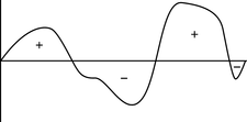
Figure q: Area underneath the axis is considered negative.
It's important to realize that this technique gives you Δ x, not x. The v-t graph has no information about where the object was when it started.
The following are important points to keep in mind when applying this technique:
-
If the range of v values on your graph does not extend down to zero, then you will get the wrong answer unless you compensate by adding in the area that is not shown.
-
As in the example, one rectangle on the graph paper does not necessarily correspond to one meter of distance.
-
Negative velocity values represent motion in the opposite direction, so as suggested by figure r, area under the t axis should be subtracted, i.e., counted as “negative area.”
-
Since the result is a Δ x value, it only tells you \(x_{after}\)-\(x_{before}\), which may be less than the actual distance traveled. For instance, the object could come back to its original position at the end, which would correspond to Δ x=0, even though it had actually moved a nonzero distance.
Finally, note that one can find Δ v from an a-t graph using an entirely analogous method. Each rectangle on the a-t graph represents a certain amount of velocity change.

Figure r: The shaded area tells us how far an object moves while accelerating at a constant rate.
Algebraic results for constant acceleration
Although the area-under-the-curve technique can be applied to any graph, no matter how complicated, it may be laborious to carry out, and if fractions of rectangles must be estimated the result will only be approximate. In the special case of motion with constant acceleration, it is possible to find a convenient shortcut which produces exact results. When the acceleration is constant, the v-t graph is a straight line, as shown in the figure. The area under the curve can be divided into a triangle plus a rectangle, both of whose areas can be calculated exactly: A=bh for a rectangle and A=bh/2 for a triangle. The height of the rectangle is the initial velocity, v\(_{o}\), and the height of the triangle is the change in velocity from beginning to end, Δ v. The object's Δ x is therefore given by the equation Δ x = v\(_{o}\) Δ t + Δ vΔ t/2. This can be simplified a little by using the definition of acceleration, a=Δ v/Δ t, to eliminate Δ v, giving
$$Δx=v_oΔt+12aΔt^2.\; \; \text{[motion with constant acceleration]}$$
Since this is a second-order polynomial in Δ t, the graph of Δ x versus Δ t is a parabola, and the same is true of a graph of x versus t --- the two graphs differ only by shifting along the two axes. Although the figure that shows a positive v\(_{o}\), positive a, and so on, it still turns out to be true regardless of what plus and minus signs are involved.
Another useful equation can be derived if one wants to relate the change in velocity to the distance traveled. This is useful, for instance, for finding the distance needed by a car to come to a stop. For simplicity, we start by deriving the equation for the special case of v\(_{o}\)=0, in which the final velocity v\(_{f}\) is a synonym for Δ v. Since velocity and distance are the variables of interest, not time, we take the equation Δx=12aΔt\(^{2}\) and use Δ t=Δ v/a to eliminate Δ t. This gives Δ x=(Δ v)\(^{2}\)/2a, which can be rewritten as
$$v_{f}^2=2aΔx. \; \text{[motion with constant acceleration, v_o = 0]}$$
For the more general case where v\(_{o}\)≠ 0, we skip the tedious algebra leading to the more general equation,
$$v_{f}^2=v_{o}^2+2aΔx.\; \; \text{[motion with constant acceleration]}$$
To help get this all organized in your head, first let's categorize the variables as follows: Variables that change during motion with constant acceleration:
x ,v, t
Variable that doesn't change:
a
If you know one of the changing variables and want to find another, there is always an equation that relates those two:
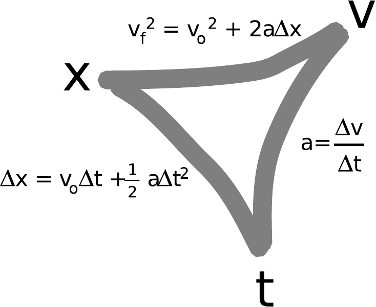
Figure s
The symmetry among the three variables is imperfect only because the equation relating x and t includes the initial velocity.
There are two main difficulties encountered by students in applying these equations:
- The equations apply only to motion with constant acceleration. You can't apply them if the acceleration is changing.
- Students are often unsure of which equation to use, or may cause themselves unnecessary work by taking the longer path around the triangle in the chart above. Organize your thoughts by listing the variables you are given, the ones you want to find, and the ones you aren't given and don't care about.
Example 8 Saving an old lady
◊ You are trying to pull an old lady out of the way of an oncoming truck. You are able to give her an acceleration of 20 m/s\(^{2}\) . Starting from rest, how much time is required in order to move her 2 m?
◊ First we organize our thoughts:
Variables given: Δ x, a, v\(_{o}\)
Variables desired: Δ t
Irrelevant variables: v\(_{f}\)
Consulting the triangular chart above, the equation we need is clearly Δx=v\(_{o}\)Δt+12aΔt\(^{2}\) , since it has the four variables of interest and omits the irrelevant one. Eliminating the v\(_{o}\) term and solving for Δ t gives Δt=2Δx/a=0.4 s .
Applications of calculus
In calculus, the area under the v-t graph between t=\(t_{1}\) and t=\(t_{2}\) is notated like this:
$$\text{area under curve} \; =Δx=∫t_1 t_2 v dt$$
The expression on the right is called an integral, and the s-shaped symbol, the integral sign, is read as “integral of ...”
Integral calculus and differential calculus are closely related. For instance, if you take the derivative of the function x(t), you get the function v(t), and if you integrate the function v(t), you get x(t) back again. In other words, integration and differentiation are inverse operations. This is known as the fundamental theorem of calculus.
On an unrelated topic, there is a special notation for taking the derivative of a function twice. The acceleration, for instance, is the second (i.e., double) derivative of the position, because differentiating x once gives v, and then differentiating v gives a. This is written as
$$a=d^2x/dt^2$$
The seemingly inconsistent placement of the twos on the top and bottom confuses all beginning calculus students. The motivation for this funny notation is that acceleration has units of m/s\(^{2}\) , and the notation correctly suggests that: the top looks like it has units of meters, the bottom seconds. The notation is not meant, however, to suggest that \(t\) is really squared.